Examples

This page reproduces the example from the README.

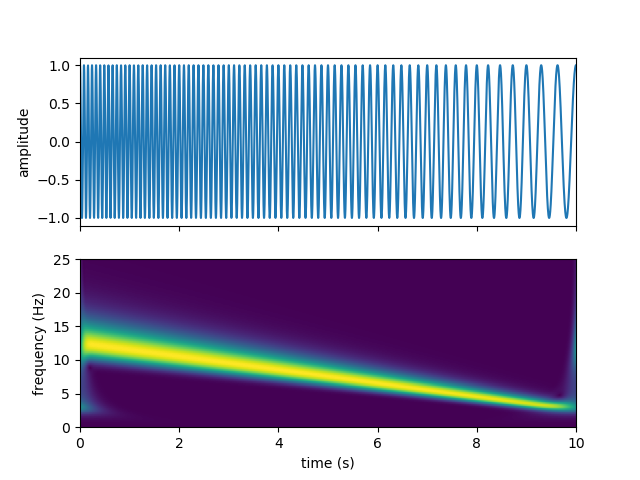
Forward Stockwell Transform

The following code generates a linear chirp, computes its Stockwell transform, and plots the time series and the resulting time-frequency spectrum:

import numpy as np
from scipy.signal import chirp
import matplotlib.pyplot as plt
from stockwell import st

t = np.linspace(0, 10, 5001)
w = chirp(t, f0=12.5, f1=2.5, t1=10, method='linear')

fmin = 0  # Hz
fmax = 25  # Hz
df = 1. / (t[-1] - t[0])  # sampling step in frequency domain (Hz)
fmin_samples = int(fmin / df)
fmax_samples = int(fmax / df)
stock = st.st(w, fmin_samples, fmax_samples)
extent = (t[0], t[-1], fmin, fmax)

fig, ax = plt.subplots(2, 1, sharex=True)
ax[0].plot(t, w)
ax[0].set(ylabel='amplitude')
ax[1].imshow(np.abs(stock), origin='lower', extent=extent)
ax[1].axis('tight')
ax[1].set(xlabel='time (s)', ylabel='frequency (Hz)')
plt.show()

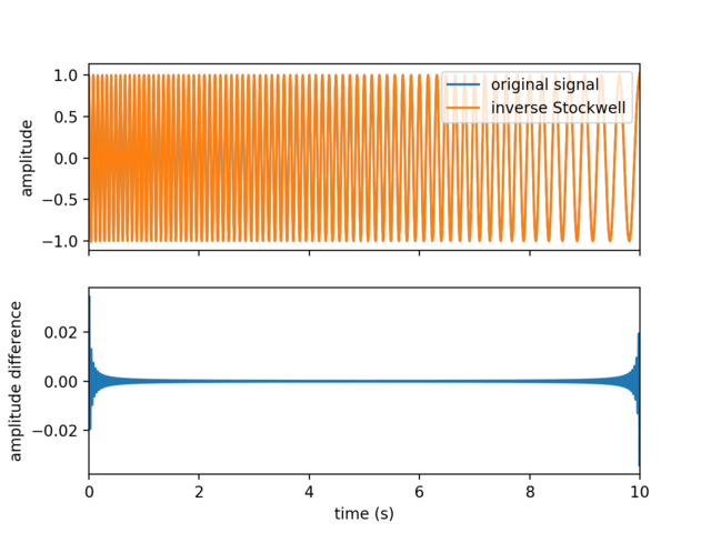
Inverse Stockwell Transform

The inverse transform recovers the original time-domain signal from its Stockwell spectrum:

inv_stock = st.ist(stock, fmin_samples, fmax_samples)
fig, ax = plt.subplots(2, 1, sharex=True)
ax[0].plot(t, w, label='original signal')
ax[0].plot(t, inv_stock, label='inverse Stockwell')
ax[0].set(ylabel='amplitude')
ax[0].legend(loc='upper right')
ax[1].plot(t, w - inv_stock)
ax[1].set_xlim(0, 10)
ax[1].set(xlabel='time (s)', ylabel='amplitude difference')
plt.show()